Introduction In July 1985, Ken Perlin introduced his much-used algorithm for producing organic randomness, now known as Perlin noise [1]. That function consists of four important subroutines:

• Random gradient vector lookup.
• S-curve evaluation.
• Grid-point dot product evaluation.
• Interpolation across all dimensions.

One can find out the basics of this algorithm from the oft-visited tutorial website "Making Noise" [2]. Assuming that you are familiar with the Perlin noise function, you may have been excited to see the 2002 Ken Perlin paper "Improving Noise" [3]. That brief report on "improved noise" gave a very elegant implementation of the classic noise algorithm useful to so many procedural methods. Other optimizations and extensions have been made to the Perlin noise algorithm for use in various settings. Among these is "simplex noise" [4][5], offered by Perlin in 2001 - a straightforward approach to quickly computing high-dimensional noise functions - and "modified noise" [6], by Marc Olano - which produces certain desirable noise properties efficiently on GPU systems. 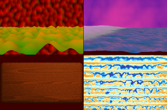Graphics using the 2002 improved noise algorithm (D Nielsen) I developed the following "dynamic noise" algorithm in March 2004. In this context, the word "dynamic" refers to the inherently mutable nature of this noise function. In other words, it moves. While rereading my senior design project from the year before (a hardware-description-language implementation of improved noise with minor novelties), I noticed I had obliquely mentioned that the noise algorithm could likely be made dynamic. With a bit of tinkering, this algorithm emerged. I do not know whether something similar has arisen any place in the field, but the function has proven useful, so it seemed time to make certain it was passed on. (All other attempts to do so have seemed unusually thwarted by the universe.) Okay, enough about myself. The general enhancement of this algorithm is noise movement without need of slicing through a higher dimension, so much less computation is required. The general drawbacks are slightly augmented memory usage as compared to traditional noise due to scaling of the gradient vectors, and use of an iterative timestepping approach that makes backtracking to a previous noise state or changing flow velocity more difficult than in the traditional approach of slicing through a higher dimension. 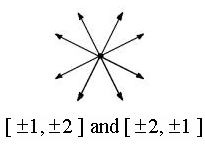Method We should begin by describing a 2D implementation of improved noise. Perlin provides code for the 3D case accompanying his 2002 brief, but leaves other cases out. We can use our own sensibilities to create a 2D case. The main difference is the set of possible gradient direction vectors. We will place them within the set {[1,2], [1,-2], [-1,2], [-1,-2], [2,1], [2,-1], [-2,1], [-2,-1]}. These vectors do not align with either the grid lines or the grid diagonals, as Perlin suggests they should not. Generating dynamic noise is very similar to making improved noise, with one primary difference: all 3-bit gradient direction vectors are scaled by an unsigned value. This produces a slightly less dense noise function, but a more controllable one. For the 2D case, we will scale the gradient vectors with a 3-bit unsigned value. The 3-bit [0..7] range simply emerged from guesswork and testing. It seems to be the smallest bit-width that produces mostly decent results, at least with a constant change factor in scale. The change in gradient vector scale per time step is stored in a 1-bit value, representing +1 or -1 change. When changing, the gradient vectors just scale up and down, up and down: 0, 1, 2, 3, 4, 5, 6, 7, 6, 5, 4, 3, 2, 1, 0, 1, 2, ... The gradient vector scale change is made based on a coin toss: true then change, else leave it alone. I believe I had also tried other nonlinear methods like bit-shifting scale and changing the scale sinusoidally to get higher-order continuity over time, but they did not work out so well. All this yields the following values in the gradient LUT for the 2D case:

• 3 bits for scale, indicating a value in range [0..7].
• 3 bits for direction, indicating [1,2], [1,-2], [-1,2], [-1,-2], [2,1], [2,-1], [-2,1], or [-2,-1].
• 1 bit for scale delta, indicating +1 or -1.

For the 3D case, four bits are needed for direction, giving 4b (direction) + 3b (scale) + 1b (scale change) = 1B. The magic is that, when gradient vectors are scaled by zero, we can swap around the direction vectors without any noticeable effect. Then, when they are rescaled, the noise function takes on the new form determined by the gradient direction vectors. As gradient vectors change scale, new vectors are always reaching zero scale, and so gradient vector swapping occurs every time step. If you are familiar with the improved noise function, this may sound pretty simple. And it is! This approach also implies the constraint that gradient direction vectors must be stored in writable memory, of course, not constants. The 1D case is trivial, and the 3D case can be extrapolated from the Perlin improved noise code and an understanding of the dynamic noise approach. Higher dimensions are not presented. 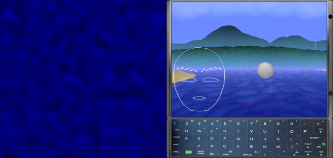Graphics using dynamic noise (D Nielsen) Economy The dynamic noise implementation presented here requires the following measures over static noise:

• The table holding permutation values must be independent of that holding gradient lookup values.
• The dot products evaluated at grid points must be scaled.
• Time changes iteratively, not as a function parameter.
• Gradient values must be updated whenever a time step occurs.

The true cost of these new requirements is small and is further diminished due to constraints and provisions already inherent in target systems. For example, a hardware implementation of the static noise function is well-suited to pipelining; therefore, it may be advantageous to place the permutation table in a processing stage independent of the table holding gradient vectors, in order to load-balance stages in the pipeline. Notice also that the gradient direction values require fewer bits per entry than do the permutation values, so that a separate gradient direction table does not require much additional memory. As an approximation, we can think of the dynamic noise function as being half the computational complexity of a comparable improved noise function. A static improved noise function on a regular grid in N-space is usually computed as an interpolation of two noise functions in (N-1)-space (except with grid-point evaluations using vectors in N-space). By reducing the dimensional requirement by one dimension, less than half of the computations are required for a dynamic noise evaluation. It is expected that dynamic noise benefits from GPU vector hardware operations, because such operations could be used to perform the grid-point dot products and scaling, and that matrix operations might be used to perform groups of vector operations for even better savings. Conclusion This algorithm is quite simple and useful, and can produce convincing results for most noisy effects, although the particular implementation given here is likely not suitable for very highend visuals due to coarse timestepping and efficient integer math. (For a critique of Perlin noise in general, see [7].) The believed enhancements that dynamic noise provides are reduced computational complexity by over half, better localized noise density conservation (so there is more of a sense of flow), and no question of slice orientation or ordered holes appearing from use of a higher dimension. This method also provides smoothly variable flow velocity when rotating a slice through a higher dimension. While the need for independence between the gradient table and the permutation table is required in this dynamic noise implementation (unlike the reusable table of static noise), a pipelined hardware implementation begs this independence anyway. A set of dynamic noise C++ classes (1D, 2D, and 3D) can be found in source code below, along with a separate Windows demonstration binary. The executable displays layered dynamic noise in various places around a scene. These files are provided for your convenience. There is no guarantee about any behavior on any system - use and modification is allowed within your own liability. noise.zip Thanks and happy coding! References [1] Perlin, K. An image synthesizer. 1985. http://portal.acm.org/citation.cfm?id=325247 [2] Perlin, K. Making noise. 2000. http://www.noisemachine.com/talk1/index.html [3] Perlin, K. Improving noise. 2002. http://mrl.nyu.edu/~perlin/paper445.pdf [4] Perlin, K. A sheet of simplex noise. 2006. http://mrl.nyu.edu/~perlin/homepage2006/simplex_noise/index.html [5] Gustavson, S. Simplex noise demystified. 2005. http://webstaff.itn.liu.se/~stegu/simplexnoise/simplexnoise.pdf [6] Olano, M. Modified noise for evaluation on graphics hardware. 2005. http://www.cs.umbc.edu/~olano/papers/mNoise.pdf [7] Cook, RL, et al. Wavelet noise. 2005. http://portal.acm.org/citation.cfm?id=1073204.1073264